CHAPTER 17

---

FURTHER REFINEMENTS: TRANSIENT BEHAVIOUR; VERY HIGH AND VERY LOW STRAIN RATES; HIGH PRESSURE

 

17.1 Transient Behaviour and Transient Maps

• Elastic deformation

• Low-Temperature plasticity

• Power-law creep

• Diffusional flow

• Construction of transient maps

17.2 High Strain-Rates

• Phonon and electron drag, and the relativistic limit

• Power-law breakdown

• Adiabatic shear

• Deformation maps extended to high strain-rates

17.3 Very Low Stresses

• Threshold stresses for power-law creep

• Diffusional flow at low stresses

• The threshold stress in pure materials

• Mobility-controlled diffusional flow in alloys and compounds

17.4 The Effect of Pressure on Plastic Flow

• Effect of pressure on the ionic volume, lattice parameter and moduli

• Effect of pressure on low-temperature plasticity

• The effect of pressure on creep

• Incorporation of pressure dependence into deformation maps

References for Chapter 17

 

The maps shown so far in this book are based on simplified rate-equations which describe behaviour at steady structure or at steady state (Chapters 1 and 2), ignoring the effects of work-hardening and of transient creep. They ignore, too, deformation mechanisms which become important when strain rates are very large (among them phonon drag and adiabatic heating) or very small (such as threshold effects associated with diffusional flow), and the influence of large hydrostatic pressures. This was done because the data for these mechanisms are so meagre that their rates, and even their placings on the maps, are often uncertain. But as a better understanding of them becomes available they can be included. In this chapter we discuss the present level of understanding, and show maps illustrating their characteristics.

 

17.1 TRANSIENT BEHAVIOUR AND TRANSIENT MAPS

<Back to Top>

When strains are small, as they are in service life of most engineering structures, the steady-state approximation is a poor one. At ambient temperatures, metals work-harden, so that the flow stress (at a given strain-rate) changes with strain. At higher temperatures most materials show primary or transient creep as well as steady-state flow; if small strains concern us we cannot neglect their contribution.

Flow at steady structure or steady state is described (Chapter 1) by an equation of the form:

(17.1)

The state variables S_i (dislocation density and so forth) do not appear as independent variables because they are either fixed, or uniquely determined by σ_s and T. But during non-steady flow the state variables change with time or strain:

Si = Si(t or γ)

(17.2)

and a more elaborate constitutive law is needed, containing either time t or a strain γ as an additional variable:

(17.3)

If this law is integrated to give:

γ = F(σs, T, t)

(17.4)

we can construct maps, still using σ_s/μ and T/T_M as axes, but with contours showing the strain γ accumulated during the time t. Such maps can include work-hardening, and both transient and steady state creep (Ashby and Frost, 1976) [1].

In doing this, we lose some of the generality of the steady-state maps. The strain-rate (which is used as the dependent variable in the steady-state maps) is a differential quantity which depends only on the current structure (S_i) of the material. The strain (which is the variable we use in the transient maps) is an integral quantity: it depends not on the current structure, but on its entire history. As a result, the constitutive laws we use are largely empirical, and the maps refer to monotonic loading at constant temperature only.

We start by listing the equations used to construct transient maps for a stainless steel, and then show three examples of them. They are computed from the data listed in Table 17.1. An application of such maps is described in Chapter 19, Section 19.3.

 

Elastic deformation

A stress σ_s produces an elastic strain:

(17.5)

Since we are now concerned with strain (not strain-rate), this elastic contribution must be added to the plastic strain to calculate the total strain.

 

Low-temperature plasticity

<Back to Top>

Polycrystal stress-strain curves can, in general, be fitted to a work-hardening law, which for tensile straining, takes the form:

where ε_p is the plastic tensile strain. Inverting, and converting from tensile to equivalent shear stress and strain, gives:

where

(17.6)

and σ_0s is the initial shear strength. Data are available for many metals and alloys. Those for Type 316 stainless steel are listed in Table 17.1.

 

TABLE 17.1 Data for Type 316 stainless steel

 

Power-law creep

<Back to Top>

  When an intrinsically soft material such as a metal is loaded, dislocations are generated and the material usually work-hardens. If the stress is now held constant these dislocations rearrange, finally attaining a steady structure, and the sample creeps at a steady state. During the rearrangement, the sample creeps faster than at steady state. This normal transient has been studied and modelled by Dorn and his co-workers (Amin et al., 1970 [2]; Bird et al., 1969 [3]; Webster et al., 1969 [4]).

            On loading an intrinsically hard material (Si, Ge, ice, probably most oxides, silicates, etc.) it appears that too few dislocations are immediately available to permit steady flow. As they move they multiply; during this process the creep-rate increases to that of the steady state. This inverse transient has been studied and modelled by Li (1963) [5], Alexander and Haasen (1968) [6], Gilman (1969) [7] and others. We shall restrict the discussion to that of normal transients. Many engineering texts and papers use a law:

(17.7)

when n and q are positive and greater than unity and σ and ε are the tensile stress and creep strain, and t is time. Differentiating and rearranging gives laws of the two forms:                      

(17.8)

Though analytically convenient, these laws are physically unsound. Both predict infinite creep rates at zero time (or strain) and no steady state; and, like all integral formulations, they cannot predict the effect of changes of stress (see the discussion of Finnie and Heller, 1959 [8]). Some of these difficulties are removed in the formulation of Dorn and his co-workers (Webster et al., 1969 [4]; Amin et al., 1970 [2]). They demonstrate remarkable agreement of creep data for Al, Mo, Ag, Fe, Cu, Ni, Nb and Pt with the creep law.    

(17.9)

where is the steady-state creep-rate, ε_t is the total transient strain, and C is a constant. We shall use this equation to construct maps, though it, too, is incapable of describing transient behaviour due to change of stress during a test.

Converted to shear stress and strain-rate, eqn. (17.9) becomes:

(17.10)

where is the steady-state strain-rate (and thus is identical with the rate used to construct the steady state maps, eqn. (2.21)), and . Data for Type 316 stainless steel are given in Table 17.1.

 

Diffusional flow

In a pure, one-component system, there is a small transient associated with diffusional flow. On applying a stress, grain boundary sliding generates an internal stress distribution which decays with time, ultimately reaching the steady-state level. The transient strain must be of the same order as the elastic strain σ_s/μ (since it is associated with the redistribution of internal stresses). The time constant is determined by the relaxation process involved; in this case, diffusion over distances comparable with the grain size, giving a relaxation time of about where is the steady-state strain-rate by diffusional flow and thus is identical with the rate used to construct the steady-state maps, eqn. (2.29). The strain then becomes:

(17.11)

This transient involves no new data. In alloys, larger transients with larger relaxation times, associated with the redistribution of solute by diffusion, appear. We shall not consider them here.

 

Construction of transient maps

<Back to Top>

  Figs. 17.1, 17.2 and 17.3 show transient maps for Type 316 stainless steel with a grain size of 100 µm. The first shows the areas of dominance of each mechanism after a time of 10⁴ s (about 3 hours); the second after a time of 10⁸ s (about 3 years), the third after 10⁹ s (30 years).

Within a field, one mechanism is dominant: it has contributed more strain to the total than any other. Superimposed on the fields are contours of constant shear strain: they show the total strain accumulated in the time to which the map refers: 10⁴, or 10⁸ or 10⁹ s in these examples.

The maps show an elastic field; within it, the elastic strain exceeds the total plastic strain (steady plus transient) due to all mechanisms. Above it lies the field of low-temperature plasticity; the spacing of the strain contours reflects work-hardening. The power-law creep and diffusional flow fields occupy their usual relative positions, but the boundaries separating them from each other and from the other mechanisms move as strain accumulates with time, because the various transients have different time constants.

An example of the use of these maps is given in Chapter 19, Section 19.3.

 

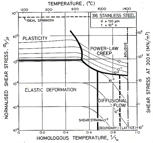
Fig. 17.1. A transient map for Type 316 stainless of grain size 100 µm, for a time of 10⁴ s (about 3 hours).

 

 

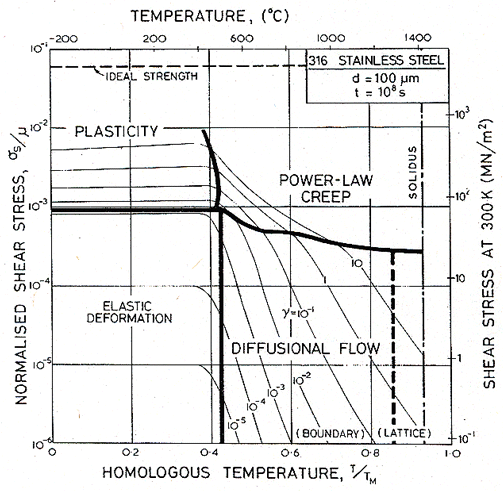
Fig. 17.2. As Fig. 17.1, but for a time of 10⁸ s (about 3 years).

 

 

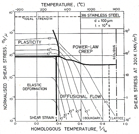
Fig. 17.3. As Fig. 17.1, but for a time of 10⁹ s (about 30 years).

 

17.2 HIGH STRAIN-RATES

Under impact conditions, and in many metalworking operations (Chapter 19, Section 19.3), strain-rates are high. They lie in the range 1/s to 10⁶/s, well above that covered by the maps shown so far. In this range, phonon and electron drags and relativistic effects can limit dislocation velocities at low temperatures; and at high, the power law which describes creep breaks down completely. Further, if the material is deformed so fast that the heat generated by the deformation is unable to diffuse away, then it may lead to a localization of slip known as adiabatic shear.

Phonon and electron drags, and power-law breakdown, are easily incorporated into deformation maps by using the rate equations given in Chapter 2. The main problem is that of data: there are very few reliable measurements from which the drag coefficient B, and the power-law breakdown coefficient α', can be determined.

 

 

Phonon and electron drag, and the relativistic limit

<Back to Top>

A moving dislocation interacts with, and scatters, phonons and electrons. If no other obstacles limit its velocity, a force σ_sb per unit length causes it to move at a velocity:

(17.12)

As the temperature increases, the phonon density rises, and the drag coefficient, B, increases. Experimental data (for review, see Klahn et al., 1970 [9] and Kocks et al., 1975 [10]) show much scatter, but are generally consistent with a drag coefficient which increases linearly with temperature:

(17.13)

where B_e is the electron drag coefficient, and B_p is the phonon-drag coefficient at 300 K.

B can be measured by direct observation of dislocation motion during a stress pulse, and can be inferred from measurements of internal friction, and from tensile or compression tests at very high strain rates. The three techniques, properly applied, show broad agreement (Klahn et al., 1970) [11]. For the metals and ionic crystals for which measurements exist, B increases from about 10^-5 Ns/m² at 4.2 K to about 10^-4 Ns/m² at room temperature. Using the Orowan equation (eqn. (2.2)), we find:

The high strain-rate experiments of Kumar et al. (1968) [12], Kumar and Kumble (1969) [13] and of Wulf (1979) [14] allow the difficult term ρb²μ/B_p to be evaluated; in all three sets of experiments the result is close to 5 x 10⁶ /s at room temperature. Combining these results gives an approximate rate-equation for phonon plus electron drag:

(17.14)

where is measured in units of s^-l. This equation has been used in constructing the maps described below.

As the dislocation velocity approaches that of sound, the stress required to move it increases more rapidly. This is in part due to the relativistic constriction of the strain field which causes the elastic energy to rise steeply, imposing a limiting velocity, roughly that of shear waves, on the moving dislocation. There is evidence (Kumar et al., 1968) [12] that the mobile dislocation density, too, rises towards a limiting value, so that, from eqn. (2.2) an upper limiting strain-rate, exists which we take to be 10⁶ s^-l. Then the approach to this limit is described by the relativistic correction to the drag equation:

(17.15)

These equations must be regarded as little more than first approximations, and they are fitted to minimal data. But they serve to show, roughly, the regimes on deformation maps in which the mechanisms have significant influence.

 

Power-law breakdown

The transition from pure power-law creep to glide-controlled plasticity was described in Chapter 2, Section 2.4. An adequate empirical description is given by eqn.(2.26), which reduces, at low stresses, to the simple power-law of eqn.(2.21). The important new parameter is α', the reciprocal of the normalized stress at which breakdown occurs. Table 17.2 lists approximate values of α' derived from the data plots of previous chapters.

 

TABLE 17.2 The power-law breakdown parameter

 

Adiabatic shear

<Back to Top>

Analyses of the onset of adiabatic shear vary in generality and complexity, but almost all are based on the same physical idea: that if the loss of strength due to heating exceeds the gain in strength due to the combined effects of strain hardening and of strain-rate hardening (which are locally higher if deformation becomes localized), then adiabatic shear will occur (Zener and Hollomon, 1944 [15]; Baron, 1956 [16]; Backofen, 1964 [17]; Culver, 1973 [18]; Argon, 1973 [19]; Staker, 1981 [20]).

Deformation generates heat, causing the flow strength σ_y to fall. Work-hardening, or an increase in strain rate, raises σ_y. Treatments of diffuse necking (Considère, 1885 [21], for example) assume that instability starts when the rate of softening first exceeds the rate of hardening. If the current flow strength is σ_y and all work is converted into heat, then the heat input per unit volume per second is:

(17.16)

The flow strength σ_y depends on strain, strain-rate and temperature:

Instability starts when dσ_y = 0, that is, when:

(17.17)

This equation is the starting point of most treatments of adiabatic localization (see, for instance, Baron, 1956 [16]; Culver, 1973 [18] or Staker, 1981 [20]).

Consider first the case when no heat is lost. (For this truly adiabatic approximation to hold, the strain-rate must be higher than the value , calculated below.) At low temperatures we can assume (as Staker, 1981 [20], does) that , so that the instability condition simplifies to:

(17.18)

or, in words: work-hardening is just offset by the fall in strength caused by heating. If heating is uniform:

dq = CpdT= σydε

or

(17.19)

If work-hardening is described by a power-law:

σy = Kεm

(17.20)

we obtain the critical strain for localization under truly adiabatic conditions:

(17.21)

where

The quantity ψ is a dimensionless material property. Typically it lies in the range –0.5 to –6. The smaller number is appropriate if the yield stress varies with temperature only as the modulus does; the larger number is typical of a material with a strongly temperature-dependent yield strength, such as the b.c.c. metals below 0.1 T_M. For many engineering metals at room temperature, its value is about –3. Then the critical strain depends mainly on the current strength σ_y, the work-hardening exponent m, the specific heat C_p and the melting point, T_M.

Eqn. (17.21) defines a sufficient condition for the onset of adiabatic shear provided no heat is lost from the sample. It is the basis of the approach used by Culver (1973) [18] and Bai (1981) [22], and by Staker (1981) [20] who supports it with data on explosively deformed AISI 4340 steel, heat-treated to give various combinations of σ_y and m. But the assumption of no heat loss holds only when the rate of deformation is sufficiently large. So a second condition must also be met: that the strain-rate exceeds a critical value which we now calculate approximately.

Consider a uniform deformation (and thus heat input) but with heat loss to the surroundings at a rate (Carslaw and Jaeger, 1959 [23], or Geiger and Poirier, 1973 [24]):

(17.22)

Here k is the thermal conductivity and R a characteristic dimension of the sample (the radius of a cylindrical sample for example); α is a constant of order 2; T is the temperature of the sample and T_s is that of the heat sink.

The heat balance equation now becomes:

(17.23)

where V is the volume of the sample and A its surface area (Estrin and Kubin, 1980 [25], for example, base their analysis on this equation). Taking A/V = 2/R we find:

(17.24)

Now the factor (C_pR²)/(2αk) = τ is the characteristic time (in seconds) for thermal diffusion to occur and is almost independent of temperature except near 0 K (it depends only on the temperature dependencies of k and C_p). Eqn. (17.24) now becomes:

(17.25)

If the critical strain for adiabatic shear is ε_c, we may write:

Heat loss to the surroundings is significant only if the second term on the left-hand side of eqn. (17.25) becomes comparable to, or larger than, the first; adiabatic conditions therefore apply when:

Using eqn. (17.21), we find the minimum strain-rate for adiabatic conditions to be, approximately:

(17.26)

At an approximate level, then, adiabatic shear is expected when two conditions are met simultaneously: the strain must exceed the critical strain given by eqn. (17.21) and the strain-rate must exceed the critical strain-rate given by eqn. (17.26). In reality, shear localization can occur even when there is heat loss. Analyses which include it are possible (Estrin and Kubin, 1980) [25] but are complicated, and, at the level of accuracy aimed at here, unnecessary.

 

Deformation maps extended to high strain-rates

<Back to Top>

Using the equations and data developed above, the influence of drag (eqn. (17.14)), or of relativistic effects (eqn. (17.15)) and of adiabatic heating (eqn. (17.26)) can be incorporated into any one of the four types of map shown in Chapter 1. The first two are straightforward; the last requires further explanation.

The parameters R and α which enter eqn. (17.26) are poorly known. But if in some standard state (say, room temperature) it is found that adiabatic localization occurs at a given strain rate , then in some other state (say 4.2 K) it will occur at the strain-rate where:

(17.27)

where the superscript ⁰ refers to the standard state and the unsuperscripted parameters are the values in the other state. We have used the fact that commercially pure titanium at room temperature shows adiabatic localization at strain-rates above 10² /s (Winter, 1975 [26]; Wulf, 1979 [14]; and Timothy, 1982 [27]) to construct maps (Fig. 17.4) which show the field in which it will occur. The most useful is that with axes of strain-rate and temperature (Fig. 17.4); it displays most effectively the region in which high strain-rate effects are unimportant. The same information can, of course, be cross-plotted onto the others.

The maps are based on data described in Chapter 6, and on those listed in Table 17.3. In addition to the usual fields, they show a regime of drag-controlled plasticity (eqn. (17.14)), the relativistic limit (eqn. (17.15)) and the regime in which adiabatic heating can cause localization (eqn. (17.26)). Adiabatic localization, of course, can occur in compression or torsion, as well as in tension; but in tension the simple necking instability may obscure the adiabatic localization because it occurs first. Further details and examples are given by Sargent and Ashby (1983) [28].

 

TABLE 17.3 Further material data for commercial-purity titanium

 

 

TABLE 17.4 Apparent threshold stresses for creep in pure metals

(a) Grain size = 1.65 x mean linear intercept.

(b) Threshold stress in shear ( when the tensile threshold σ₀ is given).

(c) Shear moduli at the test temperature calculated from data listed in Table 4.1, 5.1 and 6.1.

 

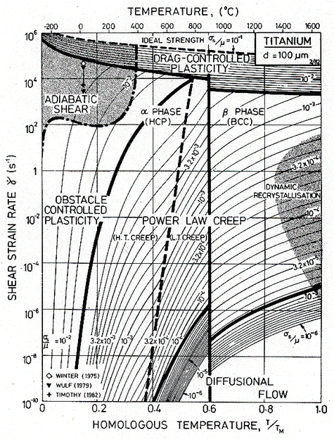
Fig. 17.4. A strain-rate/temperature map for titanium, showing the fields of drag-controlled plasticity and adiabatic shear. The relativistic limit is coincident with the top of the diagram.

 

17.3 VERY LOW STRESSES

At very low stresses there is evidence that the simple rate equations for both power-law creep (eqn. (2.21)) and for diffusional flow (eqn. (2.29)) cease to be a good description of experiments. For pure metals the discrepancies are small, but for metallic alloys, and for some ceramics, they can be large. Most commonly, the strain-rate decreases steeply with stress at low stresses, suggesting the existence of a "threshold stress" below which creep ceases, or, more accurately, a stress below which the creep-rate falls beneath the limit of resolution of the experiment (typically 10^-9 /s).

Observed "threshold stresses", τ_tr, for pure metals, alloys and one ceramic are listed in Tables 17.4 and 17.5. In pure metals, τ_tr increases with decreasing grain size and with decreasing temperature, and is of general order 5 x 10^-6 μ. In alloys containing a stable dispersion (of ThO₂, or of Y₂O₃, for example) it can be 10 to 100 times larger.

 

Threshold stresses for power-law creep

<Back to Top>

In single crystals or large-grained polycrystals, power-law creep dominates for all interesting stresses. In pure metals the power law is well-behaved at low stresses. A fine dispersion of second phase introduces an apparent threshold stress, below which creep is too slow to measure with ordinary equipment. The most complete studies are those of Dorey (1968), Humphries et al. (1970) and Shewlelt and Brown (1974, 1977) [39, 40] who introduced up to 9% of SiO₂, Al₂O₃ and BeO into single crystals of copper. They found that, on introducing the dispersion, the power n rose from the value characteristic of pure copper (about 5) to a much larger value (10 or more) at low stresses, giving the appearance of a threshold on a log vs. 1og σ diagram. The data in these tests extends down to a strain rate of 10^–6/s, at which apparent thresholds of order 10^-4 μ were observed.

At low temperatures, plastic flow in a dispersion-hardened crystal requires a stress sufficient to bow dislocations between the dispersed particles; if their spacing is l, this Orowan stress is roughly:

(17.28)

(Chapter 2 and Table 2.1). Shewfelt and Brown demonstrate that if dislocations can climb round particles instead of bowing between them, then flow is possible at a stress as low as one-third of this, so that a creep threshold of will appear (where μ, of course, is the modulus at the test temperature). Their data, and those of Dorey (1968) and of Humphries et al. (1970) are consistent with this prediction.

The power-law behaviour of coarse-grained polycrystals is more complicated (Lund and Nix, 1976 [41]; Lin and Sherby, 1981 [42]). As with single crystals, a stable dispersion introduces an apparent threshold. In some instances it has the characteristics described above: the creep-rate becomes too small to measure below about . But in others, perhaps because of the stress-concentrating effect of grain boundary sliding or the influence of a substructure created by previous working, the threshold is not quantitatively explained.

In fine-grained polycrystals there is a further aspect. Creep does not stop when power-law creep is suppressed because it is replaced by diffusional flow. This mechanism, too, is retarded by alloying, but to a lesser degree than power-law creep. For this reason, diffusional flow at low stresses is of particular interest to us here.

 

 

 Diffusional flow at low stresses

When a grain or phase boundary acts as a sink or source for a diffusive flux of atoms, the flux has its sources and sinks in boundary dislocations which move in a non-conservative way in the boundary plane. Electron microscopy reveals dislocations of the appropriate kind (Gleiter, 1969 [43]; Schober and Balluffi, 1970 [44]) which multiply by the action of sources, so that their density increases with the stress up to about 10⁷ m/m². Both theory and experiment show that their Burger's vectors b_b are not lattice vectors (they are smaller) and therefore that they are constrained to remain in the boundary plane when they move.

The model for diffusional flow must now be modified in two ways. First, one must ask how its rate is changed by the presence of discrete sinks and sources. The answer (Arzt et al., 1982) [45] is that the change is negligible unless the density of boundary dislocation is exceedingly low; we shall ignore it here. But second, one must ask how the mobility of defects influences the creep-rate. The answer is that in pure metals of normal grain size, the mobility is high; and the creep-rate is unaffected; that is why much data for pure metals follow the simple diffusion-controlled rate-equation (2.29). Only at very low stresses does the self-stress of the boundary dislocations limit their mobility, giving a threshold. But in alloys or compounds, particularly those containing a fine, stable dispersion of a second phase, the mobility of boundary dislocations is much reduced. Then anomalously slow creep, and large apparent threshold stresses, are found. We now develop these ideas a little further.

 

The threshold stress in pure materials

<Back to Top>

A boundary dislocation of the kind of interest here cannot end within a solid. It must either be continuous, or link, at nodes (at boundary triple-junctions, for instance) to one or more other dislocations such that the sum of the Burger's vectors flowing into each node is zero. If this line now tracks across the undulating surface making up the boundary between grains, its length fluctuates, and it may be pinned by the nodes. If the self-energy of the line is:

(17.28)

then the length fluctuation, or the pinning, will introduce a threshold for dislocation motion. Both are easily modelled (e.g. Burton, 1972 [36]; Arzt et al., 1982 [45]) and lead in an obvious way to the result:

(17.29)

where d is the grain size and C is a constant close to 1. Taking b_b to be 10^-10 m (about one-third of a lattice Burger's vector), we predict threshold stresses between 2 ´ 10^-7 μ (for a grain size of 500 µm) and 10^-5 μ (for a grain size of 10 µm). They are a little smaller than those reported in Table 7.4, which probably reflect a combination of this with impurity drag, discussed next.

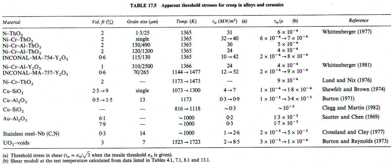
The influence of this threshold on the map for nickel is shown in Fig. 17.5. It was computed by replacing σ_s in the diffusional flow equation (eqn. (2.29)) by (σ_s — τ_tr). The map has been extended downwards by a decade in stress to allow the threshold to be seen. Over a wide range of stress, creep follows eqn. (2.29). Only near τ_tr is any change visible.

 

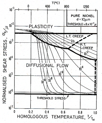
Fig. 17.5. A map for pure nickel with a threshold τ_tr of 8 ´ 10^-7 μ. The self-energy of the boundary dislocations will introduce a threshold of general magnitude .

 

Mobility-controlled diffusional flow in alloys and compounds

<Back to Top>

A solid solution, or dissolved impurities, can segregate to a boundary dislocation; then, when the dislocation moves, the segregant may diffuse along with it, exerting a viscous drag which can limit its mobility. Discrete particles of a second phase, too, interact with a boundary dislocation, pinning it, and introducing a threshold stress in much the same way that particles pin lattice dislocations and inhibit power-law creep. But because the average Burger's vector of the boundary dislocation is smaller (by a factor of perhaps 3) than that of a lattice dislocation, the extent of the segregation is less, and the pinning force is smaller. For this reason, strengthening mechanisms suppress power-law creep more effectively than diffusional flow, causing the latter to become dominant.

When the boundary-dislocation motion is impeded, part of the applied stress (or of the chemical-potential gradient it generates) is required to make the dislocations move, and only the remaining part is available to drive diffusion. The creep-rate is then slower than that given by eqn. (2.29), to an extent which we now calculate.

The velocity υ of a boundary dislocation is related to the force F per unit length acting on it through a mobility equation (cf. eqn. (2.4)):

(17.30)

Here is the part of the applied stress required to move the boundary dislocations. (We assume that, in pure shear, the boundaries are subjected to normal tractions of ± σ_s.) The strain-rate is related to b_b, υ and the density of boundary dislocations, ρ_b (a length per unit area) by:

(cf. eqn. (2.2)), where the factor 2 appears because the motion produces a normal, not a shear strain. Together these equations become:

(17.31)

This strain-rate must match that produced by the transport of matter across the grain, by diffusion, driven by the remaining part of the stress, . .From eqn. (2.29), this is:

(17.32)

Eliminating , and solving for gives:

(17.33)

This is the basic equation for diffusional flow when boundary dislocation mobility is limited (Ashby, 1969,1972) [46, 47]. Note that when M is large, the equation reduces to the classical diffusional flow law (eqn. (2.29)); but when M is small, it reduces to eqn. (17.31) with . In particular, if boundary dislocations are pinned (M = 0), creep stops. To progress further we require explicit equations for ρ_b and M.

The most reasonable assumption for the density of boundary dislocations, ρ_b, is that it increases linearly with stress (Burton, 1972 [36]; Ashby and Verrall, 1973 [48]):

(17.34)

where α is a constant of order unity. This is simply the two-dimensional analog of eqn. (2.3) for the dislocation density in a crystal.

When a solute or impurity drag restricts dislocation motion, the drag will obviously increase as the atom fraction C₀, of solute or impurities, increases. Arzt et al. (1982) [45]show that:

(17.35)

where D_s is the diffusion coefficient for the solute or impurity, and β is a constant (for a given impurity) of between 1 and 20. As an example of the influence of impurity drag, we set:

(i.e. we set D_s = D_b and ) and compute maps for nickel using eqn. (17.33), and eqn.(17.34) for diffusional flow. The results, for two grain sizes, are shown in Figs. 17.6 to 17.9. The figures illustrate how the field of diffusion-controlled flow, for which , is replaced at low stresses by one of mobility-controlled flow ("interface reaction control") for which . The size of this new field increases as the grain size decreases, and for a sufficiently large concentration C₀, or a sufficiently small diffusion coefficient D_s, it can completely replace diffusion-controlled flow.

This field rarely appears in pure metals. The small grain size necessary to observe it will not survive the tendency to grain growth at high temperatures; and the mobility of boundary dislocations is too high. Impurities lower the mobility and suppress grain growth; larger alloying additions, leading to a precipitate or a duplex microstructure, do so even more effectively. For this reason the source and sink mobility may dictate the behaviour of fine-grained two-phase superplastic alloys, which commonly show a sigmoidal stress/strain-rate relation like that shown in Fig. 17.7.

A fine dispersion of a stable phase pins boundary dislocations, so that below a threshold stress their mobility is zero. The diffusional creep behaviour is then given by eqn. (17.33) with an appropriate (nonlinear) expression for M. But at a useful level of approximation we can think of the threshold stress as subtracting from the applied stress. Then the creep-rate is given by the classical diffusional flow equation (eqn. (2.29)) with σ_s replaced by (σ_s – τ_tr); maps computed in this way are shown as Figs. 7.5 and 17.5. We anticipate that τ_tr is about one-third of the Orowan stress for boundary dislocations:

(17.36)

for the reasons given earlier in this section. Note that, because the boundary Burger's vector b_b is less than that of lattice, this threshold stress is lower, by a factor of perhaps 3, than that for power-law creep. Dispersion-hardened materials show apparent threshold stresses of general order 10^-4 μ (Table 17.5), implying an obstacle spacing of about 3000 b_b.

Apparent threshold stresses are often observed to be temperature-dependent. This can be understood (Arzt et al., 1982) [45] as a superposition of discrete obstacles and an impurity, or solute, drag: the drag causes the stress at which the strain-rate falls below the limit of resolution of the equipment to depend on temperature.

 

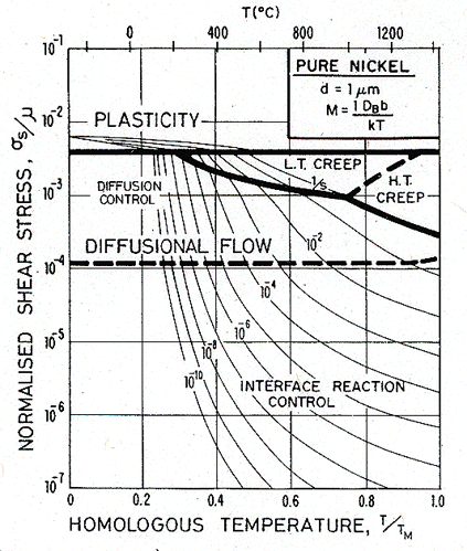
Fig. 17.6. A stress/temperature map for nickel of grain size 1 µm, with limited boundary-dislocation mobility.

 

 

Fig. 17.7. A strain-rate/stress map for nickel of grain size 1 µm, with limited boundary-dislocation mobility.

 

 

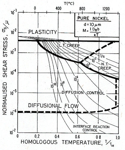
Fig. 17.8. As Fig. 17.6, but for a grain size of 10 µm.

 

 

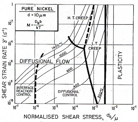
Fig. 17.9. As Fig. 17.7, but for a grain size of 10 µm.

 

17.4 THE EFFECT OF PRESSURE ON PLASTIC FLOW

In engineering design it is normal to assume that it is the shearing, or deviatoric, part of the stress field which causes flow (see Chapter 1). There is some justification for this: neither low-temperature plasticity nor creep are measurably affected by pressures of less than K/100, where K is the bulk modulus. But when the pressure exceeds this value, the flow strength is increased and the creep rate is slowed. It is still the deviatoric part of the stress field which causes flow, but the material properties (such as , ∆F, A and Q) have been altered by the pressure. Pressure must then be regarded, with temperature and shear stress, as an independent variable. In certain geophysical problems pressure is as important a variable as temperature: at a depth of 400 km below the earth's surface, for example, the pressure is about K/10, and its influence on material properties is considerable.

The influence of pressure on plastic flow has not been studied in anything like the same detail as that of temperature. But enough information exists to piece together a fairly complete picture. In this section we summarize the results required to incorporate pressure as an independent variable in computing deformation maps. Examples of their use are given in the final Case Study of this book (Section 19.8).

 

Effect of pressure on the ionic volume, lattice parameter and moduli

<Back to Top>

            In a linear-elastic solid of bulk modulus K_0, the atomic or ionic volume varies with pressure as:

,

(17.37)

and the lattice parameter a (and the Burger's vector b) as:

,

(17.38)

where Ω₀, K₀ and a₀ are the values at atmospheric pressure, p₀. Values of K₀ for elements and compounds are tabulated by Huntington (1958) [49] and Birch (1966) [50].

To first-order, the moduli increases linearly with pressure and decrease linearly with temperature. We write this in the form:

(17.39)

(17.40)

where p₀ is atmospheric pressure, which, for almost all practical purposes we can ignore.

The coefficients in the square brackets are dimensionless. Table 17.6 lists means and standard deviations of the temperature and pressure coefficients for a number of cubic elements and compounds. Most are metals, though data for alkali halides and oxides are included. The coefficients are approximately constant; when no data are available for a specific material, these constant values may reasonably be used.

 

TABLE 17.6 Temperature and pressure coefficients of the moduli and yield strength

 

Effect of pressure on low-temperature plasticity

<Back to Top>

            Experiments on a number of steels (Spitzig et al., 1975, 1976 [52, 53]; Richmond and Spitzig, 1980 [51]) have characterized the effect of a hydrostatic pressure on the flow strength. To an adequate approximation it increases linearly with pressure.

(17.41)

where (for pure iron and five steels) the dimensionless constant in square brackets has values in the range 6 to 11. The effect is far too large to be accounted for by the permanent volume expansion associated with plastic flow, and must be associated instead with a direct effect of pressure on the motion of dislocations.

This pressure-dependence can be accounted for almost entirely by considering the effect of pressure on the activation energies ∆F_p and ∆F and the strengths and which appear in eqns. (2.9) and (2.12). It is commonly found (see Kocks et al., 1975 [10], for a review) that the activation energy for both obstacle and lattice-resistance controlled glide scales as μb³ and the strengths scale as μ. For the b.c.c. metals, for example, the activation energy is close to 0.07 μb³ and the flow stress at absolute zero is close to 0.01 μ (Table 5.1, Chapter 5). As already described, both μ and b depend on pressure, μ increasing more rapidly than b³ decreases. Pressure, then, has the effect of raising both the activation energies (∆F) and the strengths ().

At absolute zero the shear stress required to cause flow is simply . Using eqn. (17.39) for the modulus, and neglecting p₀, we find by inserting the above proportionalities into eqn. (2.9) and inverting:

(17.42)

which has the form of eqn. (17.41), with:

(17.43)

Values of both dimensionless quantities are listed in Table 17.6 for variety of materials. The calculated values range from 2 to 9 compared with the measured coefficient of 6 to 11, but the measurements, of course, were made at room temperature—about 0.2 T_M for many of the listed materials. When a correction for this is made (Ashby and Verrall, 1977) [54], closer agreement is obtained.

There are other contributions to the pressure-dependence of low-temperature plasticity, but they appear to be small. The presence of a dislocation expands a crystal lattice, partly because the core has a small expansion associated with it (about 0.5 Ω per atom length) and partly because the non-linearity of the moduli causes any elastic strain-field to produce an expansion (Seeger, 1955 [55]; Lomer, 1957 [56]; Friedel, 1964 [57]). It is this second effect which is, in general, the more important. The volume expansion per unit volume of uniformly strained material is roughly:

(17.44)

where ∆E^el is the elastic energy associated with the strain-field. If the activation energy which enters the rate-equations is largely elastic in origin (as it appears to be) then during activation there is a small temporary increase in volume, ∆V. A pressure further increases the activation energy for glide by the amount p∆V. But when this contribution is compared with that caused by the change in moduli with pressure (eqn. (17.42)) it is found to be small. The influence of pressure on the low-temperature plasticity, then, is adequately described by eqn. (17.41). A pressure of 0.1 K₀ roughly doubles the flow strength.

 

The effect of pressure on creep

<Back to Top>

  There have been a limited number of creep tests in which pressure has been used as a variable; they have been reviewed by McCormick and Ruoff (1970) [58]. Typical of them are the observations of Chevalier et al. (1967) [59], who studied the creep of indium under pressure. When the pressure was switched between two fixed values the creep-rate changed sharply but reversibly, returning to its earlier value when the additional pressure was removed.

When creep is glide-controlled, pressure should influence it in the way described in the last subsection. When, instead, it is diffusion-controlled, the main influence of pressure is through its influence on the rate of diffusion. Pressure slows diffusion because it increases the energy required for an atom to jump from one site to another, and because it may cause the vacancy concentration in the solid to decrease. The subject has been extensively reviewed by Lazarus and Nachtrieb (1963) [60], Girifalco (1964) and Peterson (1968) [61]; detailed calculations are given by Keyes (1963) [62].

The application of kinetic theory to self-diffusion by a vacancy mechanism (see, for example, Shewmon, 1963 [63]) gives, for the diffusion coefficient:

(17.45)

where α is a geometric constant of the crystal structure, and α is the lattice parameter (weakly dependent on pressure in the way described by eqn. (17.38)). The important pressure-dependencies are those of the atom fraction of vacancies, n_υ, and the frequency factor, Γ. In a pure, one-component system, a certain atom fraction of vacancies is present in thermal equilibrium because the energy (∆G_f per vacancy) associated with them is offset by the configurational entropy gained by dispersing them in the crystal. But in introducing a vacancy, the volume of the solid increases by V_f, and work pV_f is done against any external pressure, p. A pressure thus increases the energy of forming a vacancy without changing the configurational entropy, and because of this the vacancy concentration in thermal equilibrium decreases. If we take:

∆Gf = ∆Gf0 + pVf ,

(17.46)

where the subscript "0" means "zero pressure", then:

nυ = exp {-(∆Gf0 + pVf)/kT}

(17.47)

A linear increase in pressure causes an exponential decrease in vacancy concentration.

It is the nature of the metallic bond that the metal tends to maintain a fixed volume per free electron. If a vacancy is created by removing an ion from the interior and placing it on the surface, the number of free electrons is unchanged, and the metal contracts. For this reason, the experimentally measured values of V_f for metals are small: about Ω₀ where Ω₀ is the atomic volume. Strongly ionic solids can behave in the opposite way: the removal of an ion exposes the surrounding shell of ions to mutual repulsive forces. The vacancy becomes a centre of dilatation, and V_f is large: up to Ω₀ where Ω₀ is the volume of the ion removed. There are no data for oxides or silicates, but when the bonding is largely covalent one might expect the close-packed oxygen lattice which characterizes many of them to behave much like an array of hard sphere. Forming a vacancy then involves a volume expansion of Ω₀, the volume associated with an oxygen atom in the structure.

There is a complicating factor. In a multicomponent system vacancies may be stabilized for reasons other than those of entropy. Ionic compounds, for instance, when doped with ions of a different valency, adjust by creating vacancies of one species or interstitials of the other to maintain charge neutrality; pressure will not, then, change the vacancy concentration significantly. Oxides may not be stoichiometric, even when pure, and the deviation from stoichiometry is often achieved by creating vacancies on one of the sub-lattices. The concentration of these vacancies is influenced by the activity of oxygen in the surrounding atmosphere, so that the partial pressure of oxygen determines the rates of diffusion. For these reasons it is possible that the quantity V_f in eqn. (17.46) could lie between 0 and Ω₀.

The jump frequency, too, depends on pressure. In diffusing, an ion passes through an activated state in which its free energy is increased by the energy of motion, ∆G_m. The frequency of such jumps is:

Γ = v exp (–∆Gm/kT),

(17.48)

where v is the vibration frequency of the atom in the ground state (and is unlikely to depend on pressure). In moving, the ion distorts its surroundings, temporarily storing elastic energy. If all the activation energy of motion is elastic, then (by the argument leading to eqn. (17.44)) it is associated with volume expansion,

Vm = 3∆Gm/2μ

per unit volume. Taking the activation energy for motion to be 0.4 of the activation energy of diffusion, we find, typically, V_m = 0.2–0.4 Ω₀, where Ω₀ is the volume of the diffusing ion. Experimentally, V_m is a little smaller than this, suggesting that the activation energy is not all elastic.

Assembling these results we find:

D = D0(1 – 2p/3K) exp (–pV*/kT) ≈ D0 exp (–pV*/kT)

(17.49)

where D⁰ = α(a₀)²v exp – (∆G_f + ∆G_m)/kT) is the diffusion coefficient under zero pressure, and:

V* = Vf + Vm for intrinsic diffusion; V* = Vm for extrinsic diffusion.

Because experiments are difficult, there are few measurements of V*, and these show much scatter. They have been reviewed by Lazarus and Nachtrieb (1963) [60], Keyes (1963) [62], Girifalco (1964) [61], Goldstein et al. (1965) [64], Brown and Ashby (1980) [65] and Sammis and Smith (1981 [66]). Some results are summarized in Table 17.7: they lie between 0 and 2Ω₀, where Ω₀ is the volume of the diffusing ion.

When creep is diffusion-controlled, the creep-rate should scale as the diffusion coefficient. The power-law creep equation (eqn. (2.21)) then becomes:

(17.50)

where μ and b are the values at the pressure p. The diffusional flow equation (eqn. (2.29)), similarly, becomes:

(17.51)

where Ω is the atomic or ionic volume at the pressure p.

When pressures are large the creep-rate depends strongly on pressure: a pressure of 0.1 K₀ reduces the creep rate, typically, by a factor of 10. The principal contribution is that of the term involving V*, so that the "activation volume" for creep, defined by:

should be close to that for diffusion, V*. Table 17.7 shows that this is so.

 

TABLE 17.7 Activation volumes for diffusion and creep

 

Incorporation of pressure dependence into deformation maps

The information summarized above allows the effect of pressure on material properties to be incorporated into deformation maps. The quantities b, Ω, μ are calculated for the given pressure, using eqns. (17.37) to (17.39). Diffusion coefficients are corrected for pressure using eqn. (17.49), or (alternatively) the creep equations are modified to eqns. (17.50) and (17.51). Finally, the flow stress for low-temperature plasticity is replaced by that given in eqn. (17.41). The final Case Study (Section 19.8) shows maps computed in this way.

 

 

References for Chapter 17

<Back to Top>

 

1. Ashby, M.F. and H.J. Frost, The Construction of Transient Maps and Structure Maps. 1976, Cambridge University Engineering Department Report.

2. Amin, K.E., A.K. Mukherjee, and J.E. Dorn, A universal law for high-temperature diffusion controlled transient creep. J. Mech. Phys. Solids, 1970. 18: p. 413-29.

3. Bird, J.E., A.K. Mukherjee, and J.F. Dorn, Correlations Between High-Temperature Creep Behaviour and Structure, D.G.a.R. Brandon, A., Editor. 1969, Haifa University Press, Israel. p. 255-341.

4. Webster, G.A., A.P.D. Cox, and J.E. Dorn, Met. Sci.J., 1969. 3: p. 221.

5. Li, J.C.M., Acta Metallurgica (pre 1990), 1963. 11: p. 1269.

6. Alexander, H. and P. Haasen, Dislocations and plastic flow in the diamond structure. Solid State Physics, 1968. 22: p. 27.

7. Gilman, J.J., Micromechanics of Flow in Solids. 1969: McGraw-Hill.

8. Finnie, I. and W.R. Heller, Creep of Engineering Materials. 1959: McGraw-Hill.

9. Klahn, D., A.K. Mukherjee, and J.E. Dorn. in Second International Conference on the Strength of Metals and Alloys. 1970. Asilomar, California: ASM.

10. Kocks, U.F., A.S. Argon, and M.F. Ashby, Prog. Mat. Sci., 1975. 19: p. 1.

11. Kocks, U.F., The relation between polycrystal deformation and single-crystal deformation. Met. Trans., 1970. 1: p. 1121.

12. Kumar, A., F.E. Hauser, and J.E. Dorn, Viscous drag on dislocations in aluminum at high strain rates. Acta Metallurgica (pre 1990), 1968. 16: p. 1189.

13. Kumar, A. and R.C. Kumble, Viscous drag on dislocations at high strain rates in copper. Journal of Applied Physics, 1969. 40: p. 3475-80.

14. Wulf, G.L., High strain rate compression of titanium and some titanium alloys. Int. J. Mech. Sci., 1979. 21: p. 713-18.

15. Zener, C. and J.H. Holloman, Effect of strain rate upon plastic flow of steel. Journal of Applied Physics, 1944. 15: p. 22.

16. Baron, H.G., J. Iron and Steel Inst., 1956. 182: p. 354.

17. Backofen, W.A., in Fracture on Engineering Materials. 1964, A.S.M.: Metals Park, Ohio. p. 107.

18. Culver, R.S., Metallurgical Effects at High Strain Rates, ed. R.e. al. 1973: Plenum. 519.

19. Argon, A.S., in The Homogeneity of Plastic Deformation. 1973, A.S.M.: Metals Park, Ohio. p. 161.

20. Staker, M.R., The relation between adiabatic shear instability strain and material properties. Acta Met., 1981. 29: p. 683.

21. Considere, M., Annls. Ponts Chauss, 1885. 9: p. 574.

22. Bai, Y., Albuquerque Conference on High Strain Rates (to be published). 1981.

23. Carslaw, H.S. and J.C. Jaeger, Conduction of Heat in Solids. 1959, Oxford: Clarendon Press.

24. Geiger, G.H. and D.R. Poirier, Transport Processes in Metallurgy. 1973: Addison Wesley. Ch. 7, P 207, et seq.

25. Estrin, Y. and L.P. Kubin, Criterion for thermomechanical instability of low temperature plastic deformation. Scripta Metallurgica (before 1990), 1980. 14: p. 1359.

26. Winter, R.E., Adiabatic shear of titanium and polymethylmethacrylate. Philosophical Magazine( before 1978), 1975. 31(4): p. 765-73.

27. Timothy, S.P., Personal communication. 1982.

28. Sargent, P.M. and M.F. Ashby, A deformation mechanism map for III-IV compound, indium antimonide. Scripta Metallurgical, 1984. 18(3): p. 219-24.

29. Doner, M. and H. Conrad, Deformation mechanism in commercial Ti-50A (0.5 at.%O_eq) at intermediate and high temperature (0.3-0.6 T_m). Met. Trans., 1973. 4: p. 2809.

30. Harding, J., The temperature and strain rate sensitivity of alpha-titanium. Archives of Mechanics, 1975. 27: p. 5-6.

31. Tanaka, K., K. Ogowa, and T. Nojima. in IUTAM Symposium on High Strain Rate Deformation. 1978. Springer, NY.

32. Crossland, I.G., Low-stress creep of cadmium. Phys. Stat. Sol. A, 1974. 23: p. 231-5.

33. Crossland, I.G. and R.B. Jones, Grain boundary diffusion creep in magnesium. Mat. Sci., 1977. 11: p. 504.

34. Crossland, I.G. Physical Metallurgy of Reactor Fuel Elements, ed. J.E.a.S. Harris, E. C. 1975, London: Metals Society. 66.

35. Towle, D.J. 1975, University of Sheffield, England.

36. Burton, B., Interface reaction controlled diffusional creep: A consideration of grain boundary dislocation climb sources. Materials Science and Engineering, 1972. 10: p. 9.

37. Towle, D.J. and H. Jones, The creep of alpha-iron at low stresses. Acta Metallurgica (pre 1990), 1976. 24: p. 399.

38. Sritharan, T. and H. Jones, The creep of beta-Colbalt at low stresses. Acta Met., 1979. 27: p. 1293.

39. Shewfelt, R.S.W. and L.M. Brown, High-temperature strength of dispersion-hardened single cryssitals- I. Experiemntal results. Phil Mag., 1974. 30: p. 1135-45.

40. Shewfelt, R.S.W. and L.M. Brown, High-temperature strength of dislocation-hardened single crystals-II. Theory. Phil. Mag., 1977. 35: p. 945-62.

41. Lund, R.W. and W.D. Nix, High-temperature creep of Ni-20Cr-2ThO₂ single crystals. Acta Metallurgica (pre 1990), 1976. 24: p. 469.

42. Lin, J. and O.D. Sherby, Res Mechanica, 1981. 2: p. 251.

43. Gleiter, H., The mechanism of grain boundary migration. Acta Metallurgica, 1969. 17: p. 565.

44. Schober, T. and R.W. Balluffi, Quantitative observation of misfit dislocation arrays in low and high angle twist grain boundaries. Phil. Mag., 1970. 21: p. 109-24.

45. Arzt, E., M.F. Ashby, and R.A. Verrall, CUED Report. 1982, Cambridge University.

46. Ashby, M.F., On interface-reaction control of Nabarro-Herring creep and sintering. Scripta Metallurgica (before 1990), 1969. 3: p. 837.

47. Ashby, M.F., A first report on deformation-mechanism maps. Acta Metallurgica (pre 1990), 1972. 20: p. 887.

48. Ashby, M.F. and R.A. Verrall, Diffusion-accommodated flow and superplasticity. Acta Metallurgica (pre 1990), 1973. 21: p. 149.

49. Huntington, H.B., The elastic constants of crystals. Solid State Physics, 1958. 7: p. 213.

50. Birch, F., Handbook of Physical Constants. Vol. Memoir 97, Section 7. 1966: The Geological Society of America.

51. Richmond, O. and W.A. Spitzig. Pressure dependence and dilatancy of plastic flow. in Proc. l5th Int. Congress on Theoretical and Applied Mechanics. 1980. Toronto: IUTAM.

52. Spitzig, W.A., R.J. Sober, and O. Richmond, Pressure dependence of yielding and associated volume expansion in tempered martensite. Acta Met., 1975. 23: p. 885.

53. Spitzig, W.A., R.J. Sober, and O. Richmond, The effect of hydrostatic pressure on the deformation behavior of maraging and HY-80 steels and its implications for plasticity theory. Trans. Met. Soc. AIME, 1976. 7A: p. 17O3-10.

54. Ashby, M.F. and R.A. Verrall, Micromechanisms of flow and fracture and their relevance to the rheology of the upper mantle. Phil. Trans. R. Soc. Lond., 1978. A288: p. 59-95.

55. Seeger, A., The generation of lattice defects by moving dislocations, and its application to the temperature dependence of the flow-stress of FCC crystals. Phil. Mag., 1955. 46: p. 1194.

56. Lomer, W.W., Density change of a crystal containing dislocations. Phil. Mag., 1957. 2: p. 1053.

57. Friedel, J., Dislocations. 1964: Pergamon. 25.

58. McCormick, P.G. and A.L. Ruoff, in Mechanical Behaviour of Materials under Pressure, H.l.D. Pugh, Editor. 1970, Elsevier.

59. Chevalier, G.T., R. McCormick, and A.L. Ruoff, Pressure dependence of high-temperature creep in single crystals of Indium. Journal of Applied Physics, 1967. 38: p. 3697-3700.

60. Lazarus, D. and N.H. Nachtrieb, in Solids under Pressure, W.a.W. Paul, D. M., Editor. 1963, McGraw-Hill. p. 43.

61. Girifalco, L.A., in Metallurgy at High Pressures and High Temperatures, K.A.H. Gachneider, M. T. and Parlee, N. A. D., Editor. 1964, Gordon & Breach. p. 260.

62. Keyes, R.W., ed. Solids under Pressure. ed. W.a.W. Paul, D. M. 1963, McGraw-Hill. 71.

63. Shewmon, P.G., Diffusion in Solids. 1963: McGraw-Hill. 52.

64. Goldstein, J.I., R.E. Hanneman, and R.E. Ogilvie, Diffusion in the Fe-Ni system at 1Atm and 40 Kbar pressure. Trans. AIME, 1965. 233: p. 813.

65. Brown, A.M., The Temperature Dependence of the Vickers Hardness of Isostructural Compounds. 1980, University of Cambridge.

66. Sammis, C.G., J.C. Smith, and G. Schubert, A critical assessment of estimation methods for activation volume. J. Geophys. Res., 1981. 86,: p. 10707-18.

 

<Back to Top>